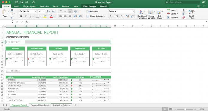
There are a lot of ways to customize the appearance of a worksheet in Excel 2010, and many of them are more useful to some people than others. For example, there are several different worksheet views that can be used, some of which are more helpful in certain situations than others. If that is the view you prefer, which is just one way to begin restoring a heavily edited spreadsheet to the default view settings. But there is another option that splits the screen, keeping a set group of rows at the top of the window as you scroll to the bottom. While this can be beneficial in certain situations, it can be annoying if you aren’t used to it. Fortunately it is a simple process to disable the split and view the spreadsheet as you normally would. Stop Splitting the Screen in Excel 2010 The split screen that I am referring to in this article looks like the image below – As you can see, there is a horizontal bar that separates the rows that I have locked in the window, while the remainder of the rows scroll normally below the split.

So continue reading below to learn how to remove this split screen on your Excel 2010 spreadsheet. Step 1: Open the Excel spreadsheet that you want to modify. Step 2: Click the View tab at the top of the window. Step 3: Click the Split button to remove the split screen.

Note that the button will be highlighted in orange before you click it, then will not be highlighted after you click it. If you are having difficulty printing in Excel, specifically fitting large spreadsheets onto fewer sheets of paper, then.

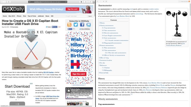
Step 1: Open the Excel spreadsheet that you want to modify. Step 2: Click the View tab at the top of the window. Step 3: Click the Split button to remove the split screen. Note that the button will be highlighted in orange before you click it, then will not be highlighted after you click it. Split View in OS X El Capitan or later lets you fill your Mac screen with two apps, without having to manually move and resize windows. Enter Split View Hold down the full-screen button in the upper-left corner of a window.

By Although zooming in and out on an Excel 2016 worksheet can help you get your bearings, it can’t bring together two separate sections so that you can compare their data on the screen (at least not at a normal size where you can actually read the information). To manage this kind of trick, split the Worksheet area into separate panes and then scroll the worksheet in each pane so that they display the parts you want to compare.

Splitting the window is easy. Look at the following figure to see an Income Analysis worksheet after splitting its worksheet window horizontally into two panes and scrolling up rows 36 through 44 in the lower pane.

Each pane has its own vertical scroll bar, which enables you to scroll different parts of the worksheet into view. The Income Analysis spreadsheet in a split window after scrolling up the bottom rows in the lower pane. To split a worksheet into two (upper and lower) horizontal panes, you simply position the cell pointer at the place in the worksheet where you want to split the worksheet and then click the Split button on the Ribbon’s View tab (or press Alt+WS). The key to the panes created with the Split button is the cell in the worksheet where you position the pointer before selecting this command button: • To split the window into two horizontal panes, position the cell pointer in column A of the row where you want to split the worksheet. • To split the window into two vertical panes, position the cell pointer in row 1 of the column where you want to split the worksheet. • To split the window into four panes — two horizontal and two vertical — position the cell pointer along the top and left edge of cell. After you split the worksheet window, Excel displays a split bar (a thin, light gray bar) along the row or column where the window split occurs. Excel add-in sql.

If you position the mouse or touch pointer anywhere on the split bar, the pointer changes from a white-cross to a split pointer shape (with black arrowheads pointing in opposite directions from parallel separated lines). You can increase or decrease the size of the current window panes by dragging the split bar up or down or left or right with the split pointer.

You can make the panes in a workbook window disappear by double-clicking anywhere on the split bar (you can also do this by selecting View→Split again).