See how Excel makes the chart wrong, but then see how to fix it. By getexcellent; 8:20 pm; WonderHowTo WonderHowTo. New to Microsoft Excel? Your browser does not currently recognize any of the video formats available. How To: Make basic balance sheet calculations in Microsoft Excel.

Last month, we that will be available as part of Office 2016. Today, we will show you how to take advantage of the Waterfall chart, one of the most popular visualization tools used in small and large businesses. With this new chart, what used to take complicated and multiple iterative steps can now be done in a few quick clicks.

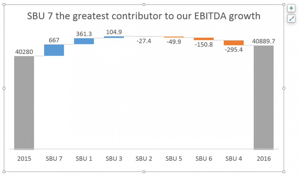
And since the Waterfall chart is built natively into Excel, you automatically get all the rich and intuitive customization, styling and formatting capabilities you’ve come to expect with the Excel charts. Waterfall charts are ideal for showing how you have arrived at a net value, by breaking down the cumulative effect of positive and negative contributions. This is very helpful for many different scenarios, from visualizing financial statements to navigating data about population, births and deaths. We added the sample workbook used to create the charts, which you can download. Getting started with the Waterfall chart A classic example for Waterfall charts is visualizing financial statements. The example below illustrates how a Waterfall chart can visually display an income statement, also known as a profit and loss statement: There are multiple ways to insert a Waterfall chart into your worksheet: the Recommended Charts tab and the All Charts tab.

You can also insert a Waterfall chart directly from the ribbon. Using the Recommended Charts feature in Excel helps you find the most effective and visually aesthetic chart for your data. Based on the range of data you have selected, the Recommended Charts feature suggests the charts that will best display your data. The Waterfall chart is recommended when the data has a column of category text, a mix of positive and negative values, and no more than a few empty value cells. The ideal dataset size for recommending charts is anywhere between 8 to 20 values, and given its most popular use case of financial statements, currency-formatted data will favor Waterfall charts. In this example, the parenthetical notation, i.e. ($2,412), is a variation of our currency formatting and denotes a negative value, -$2412.

Free download mac office 2016. To start, select your data and then under the Insert tab click the Recommended Charts button. The list of recommended charts is displayed.

Select the Waterfall recommendation to preview the chart with your selected data. The All Charts tab allows direct insertion of Waterfall charts. You can also use the ribbon to insert the Waterfall chart regardless of the data’s characteristics. Because we know that this is a popular chart, we dedicated a spot in the Chart gallery with a Waterfall icon.

Additionally, Stock Charts are also available under this drop-down because of the financial context associated with both chart types. After the new Waterfall chart is created, notice that the order in which your data is shown in your table is preserved in the chart. In this example, Gross Revenue will always be the first column since it is the first data point, followed by Rev Adjustments, and so on, until Net Income—the last data point and therefore the last column. Using subtotals as a visual checkpoint in the chart To truly make our Waterfall chart understandable, we want to set subtotals of certain accounts. Subtotals, in this case, denote balances. In any Waterfall chart, you might set a subtotal to show the absolute value rather than as a floating value relative to the previous column.